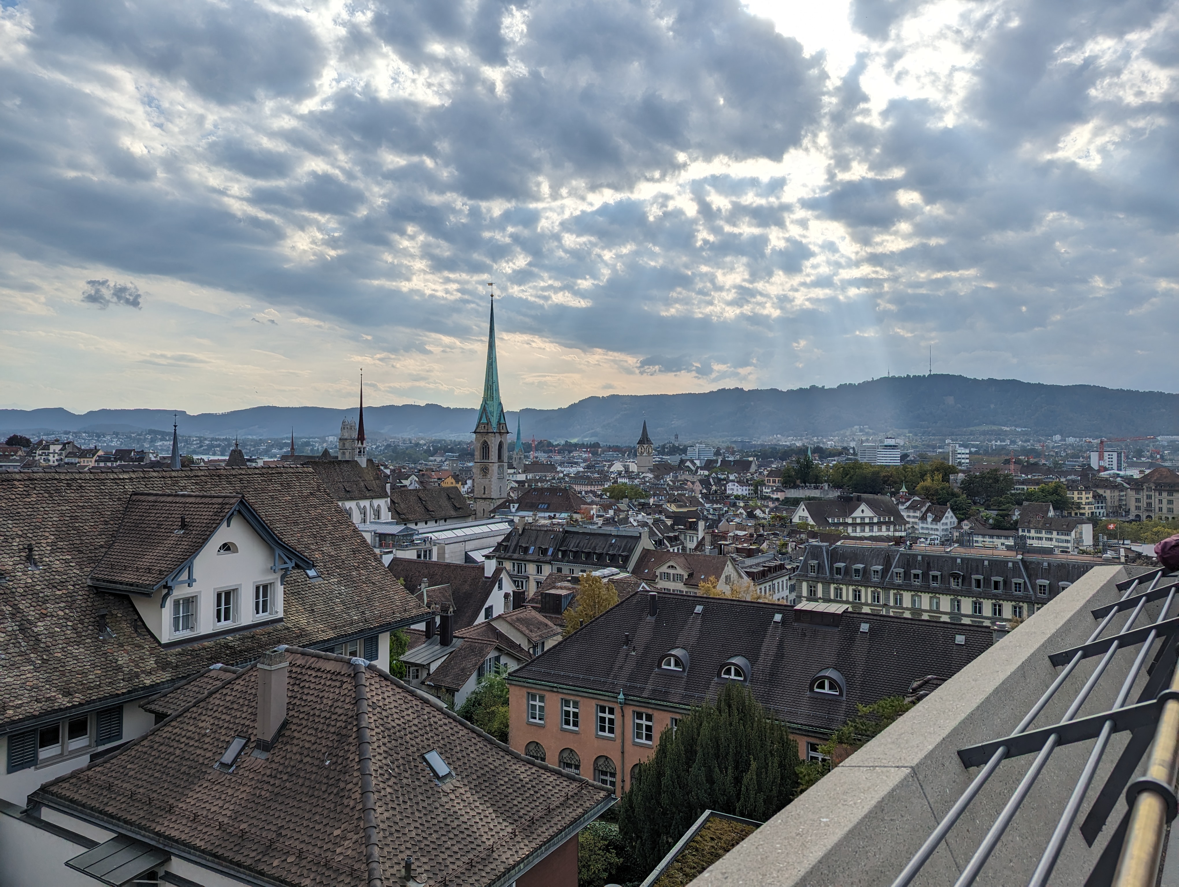
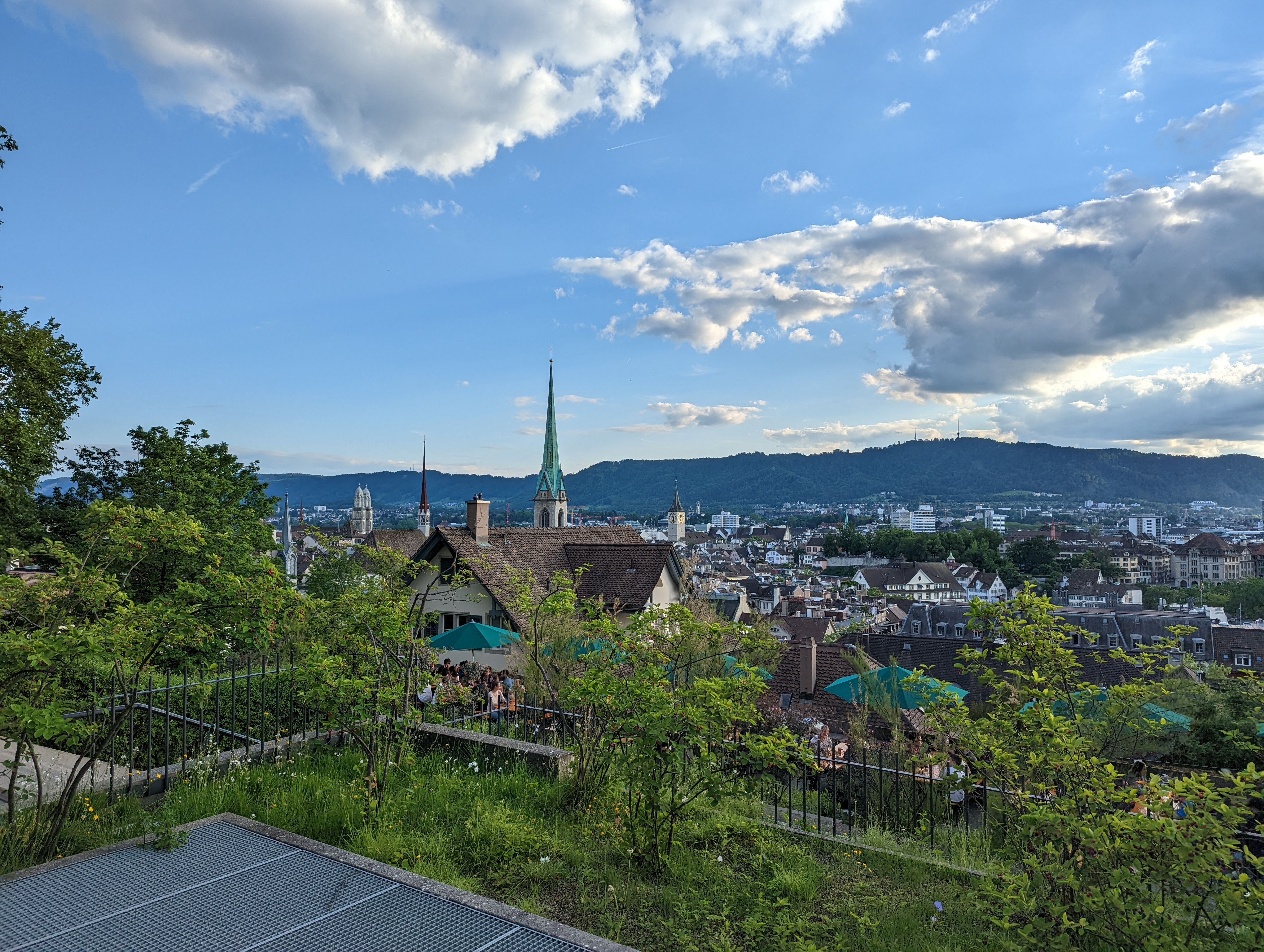
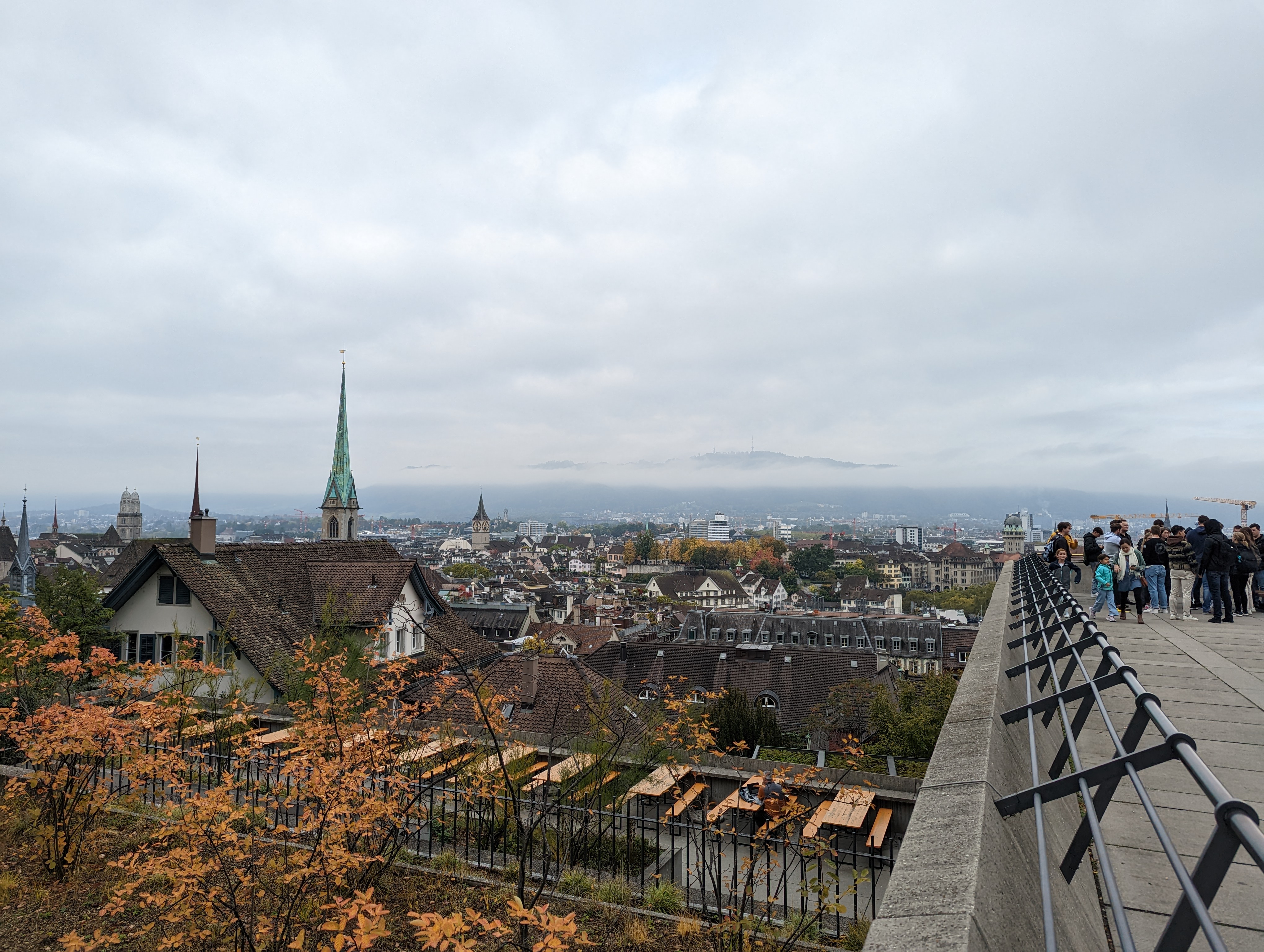
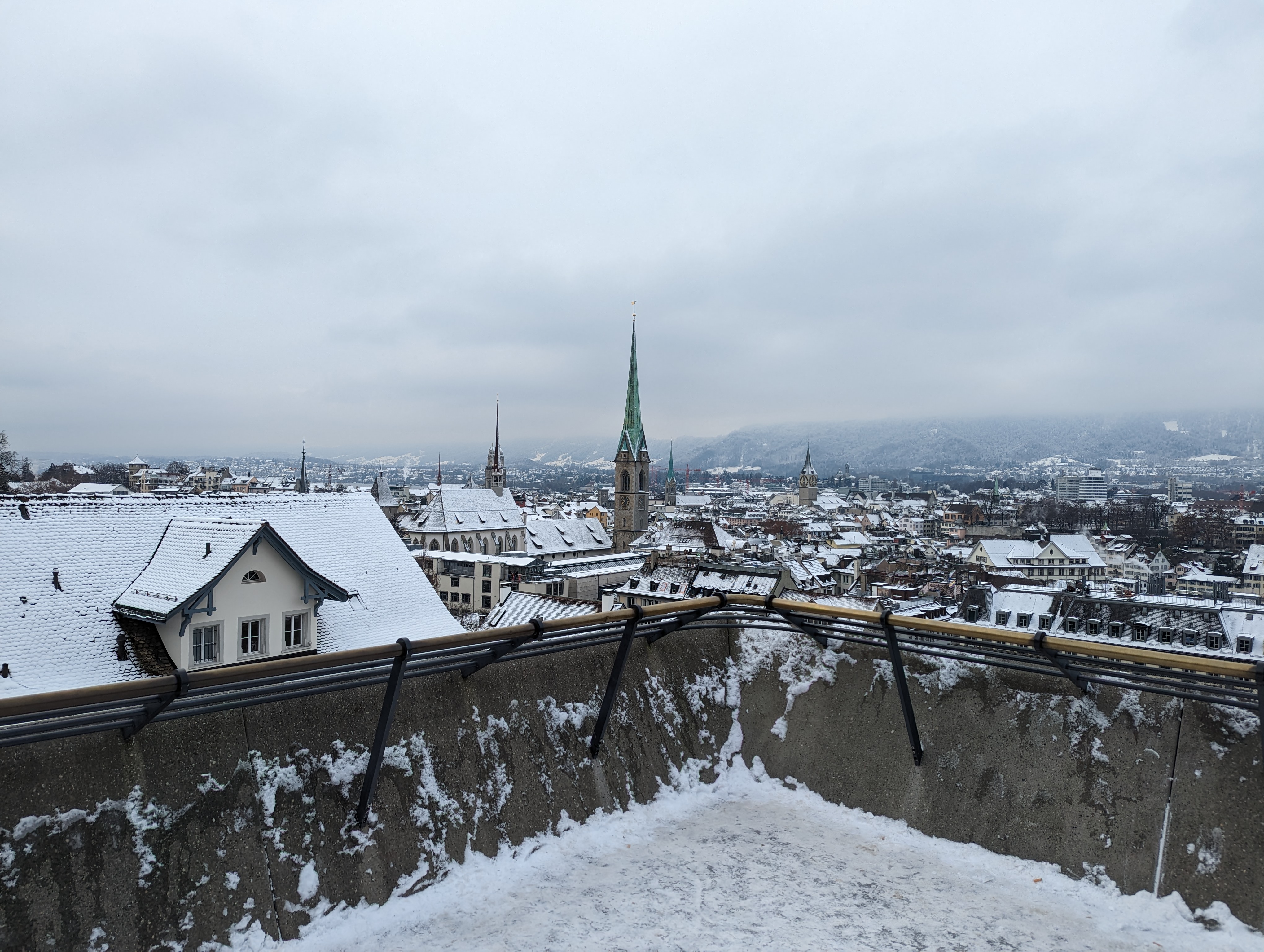
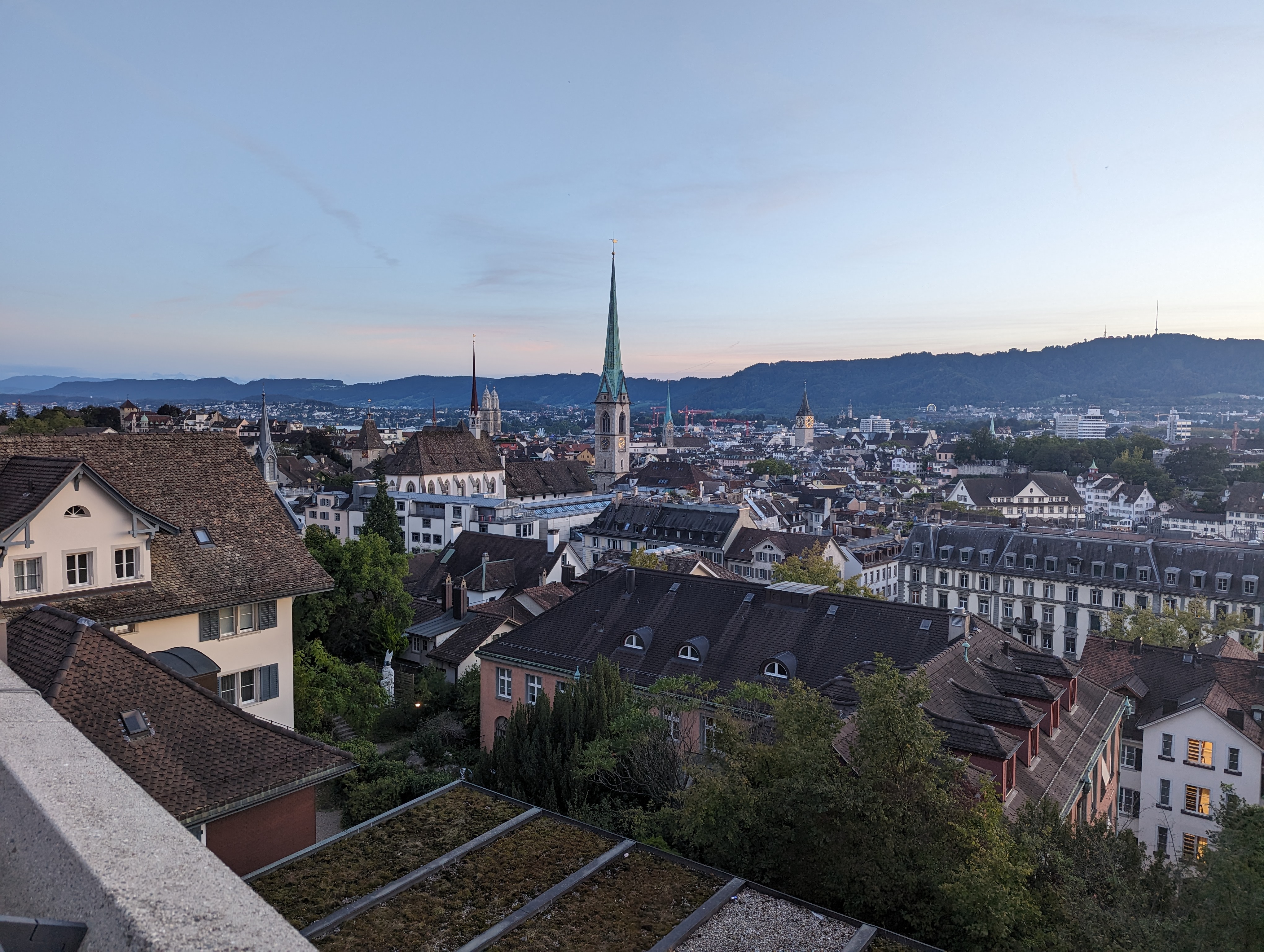
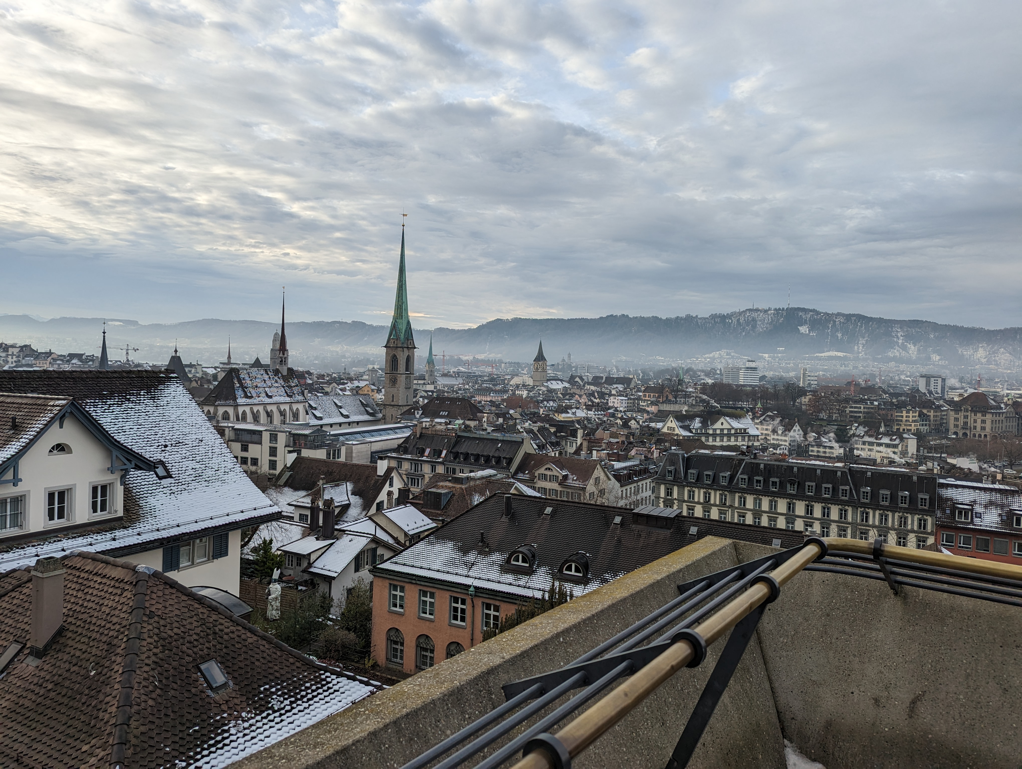
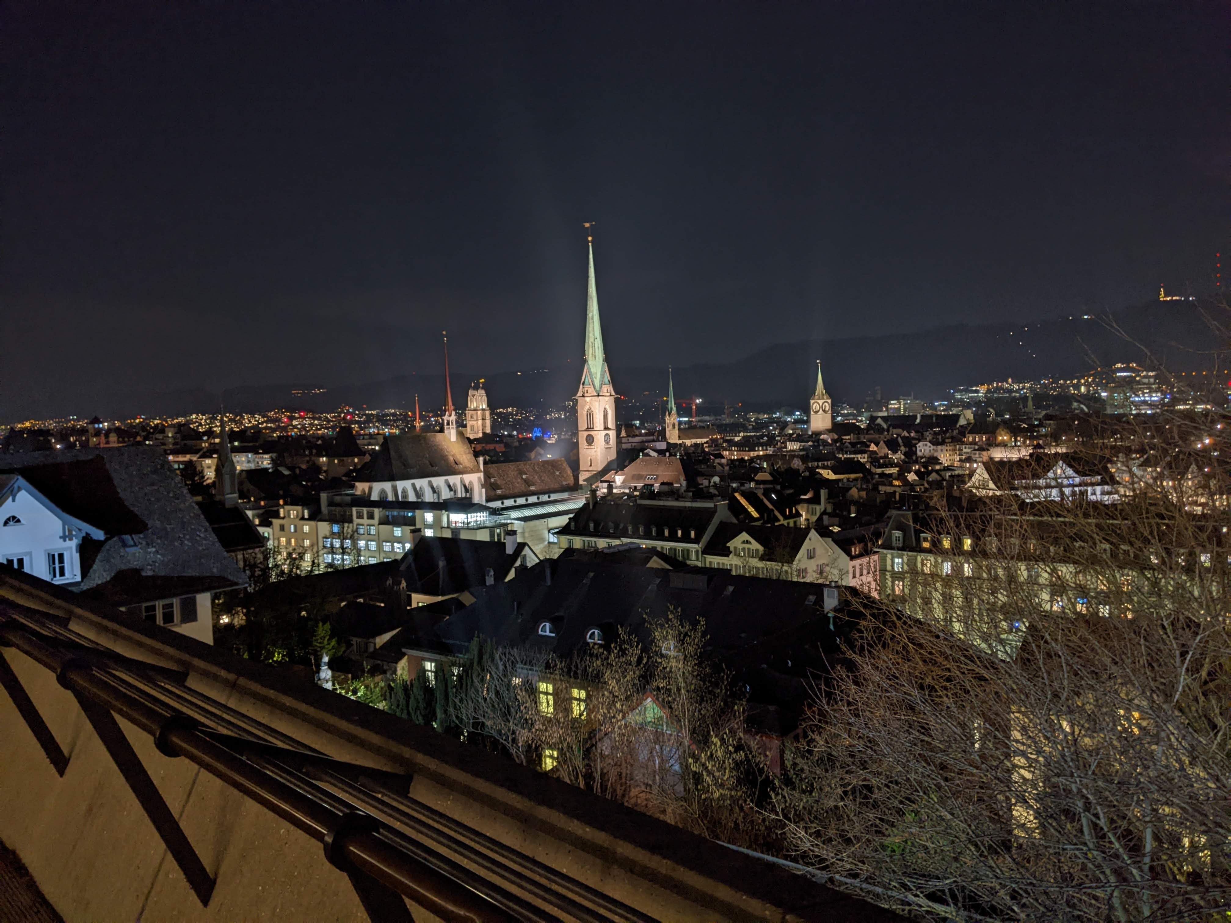
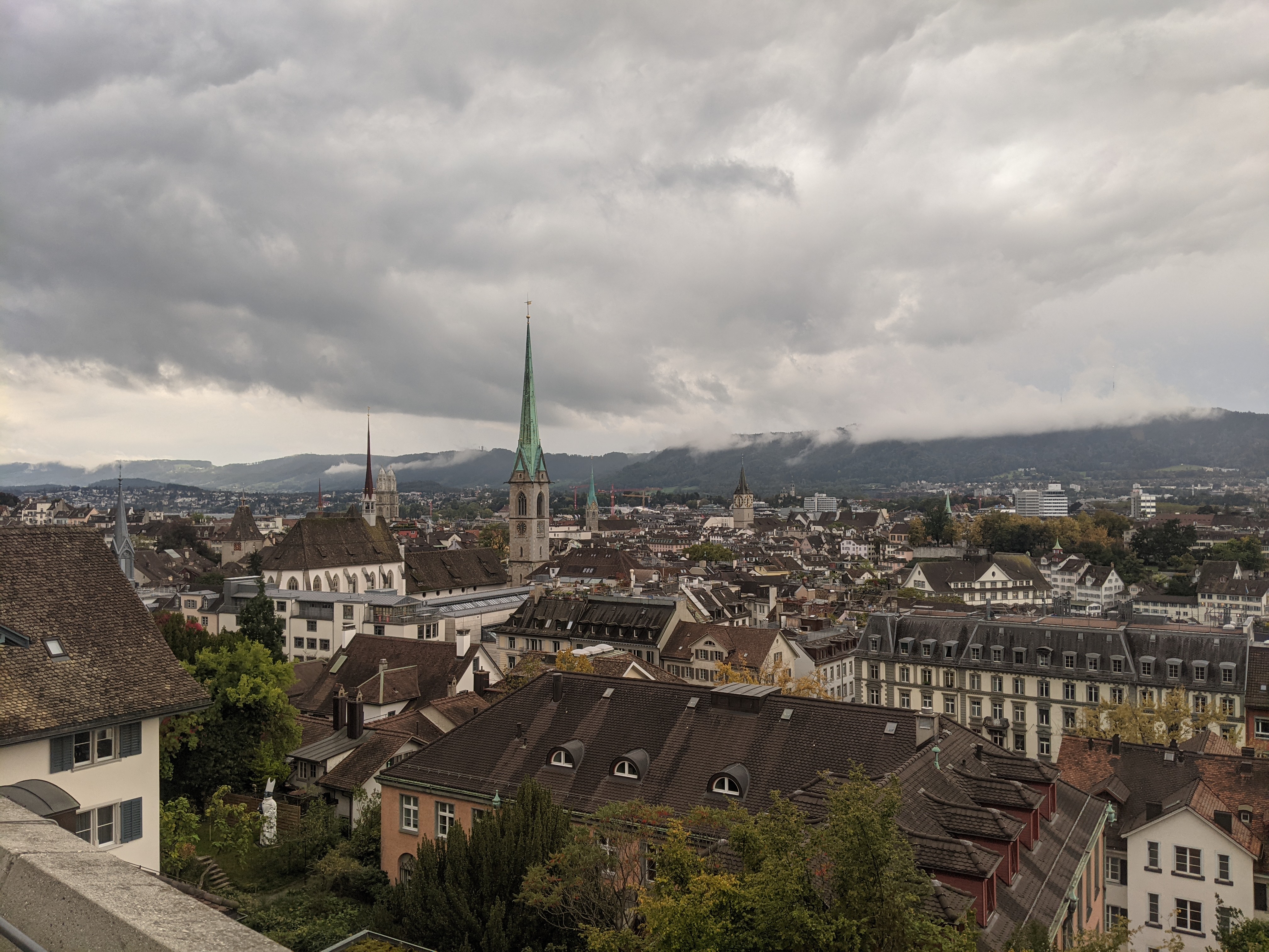
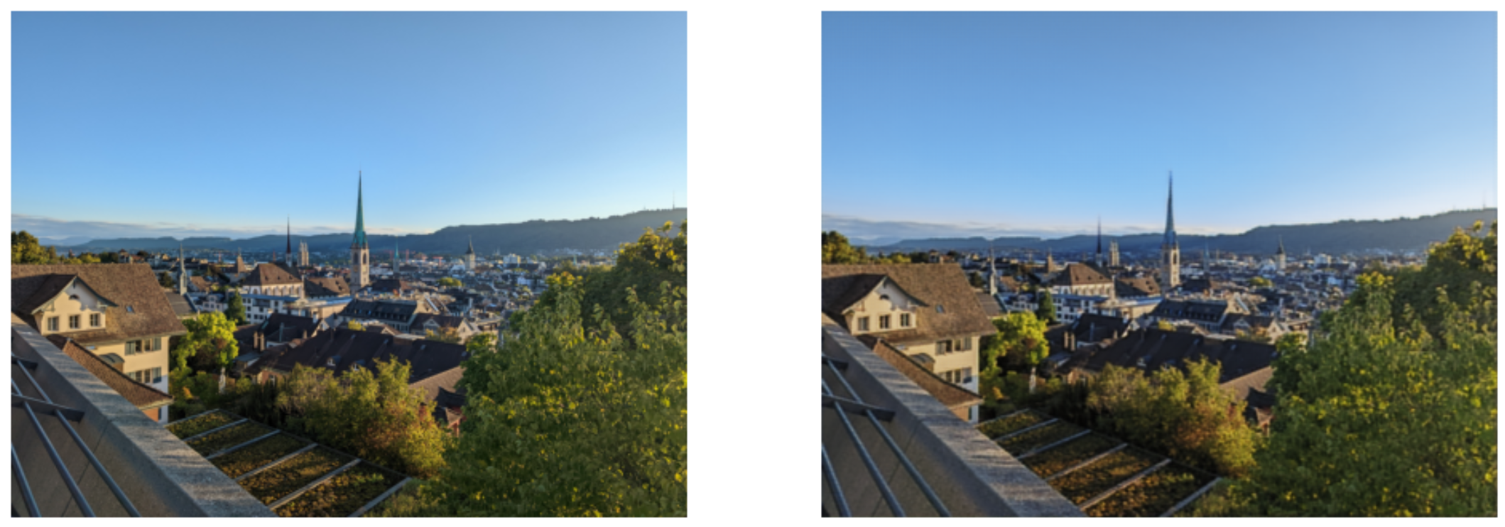
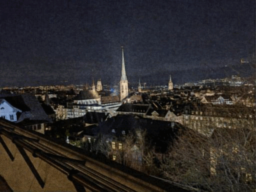
Polyterrase <3

On of the many perks of studying here at ETH Zürich is the view from Polyterasse, the terrace in front of the main building. I can still remember my first time walking by this place, and overlooking the amazing city of Zürich. Safe to say I have tons of photos of Polyterasse in my photos album taken at different times in the year and at different times of the day. I knew I wanted to play with these photos in some way or the other.

At the same time, I wanted to play around with more AI models and concepts. So why not combine the two? :D

Just as a pet project these are some of the goals I wanted to achieve:

• Filter my polyterasse photos: Having multiple photos across the years somewhere in my google photos, I wanted to be able to collect all of them together.
• Morph photos: I wanted to play around to morph them from one to another in a smooth way. Just to play around with other models and their representation.
• Stylize polyterasse: With many models performing Image to Image style transfer, I wanted to try the same for some of the pictures I took.

Code : All my code for this can be found on my Colab notebook here!

Let’s get into it shall we?

Classification / Filtering

Now Google Photos already comes up with a way to filter photos in your library either via a location, or a face, or even a tag (outdoors). Hence it was easy enough to get my photos by just searching for Polyterasse, but wheres the fun in that?

Instead I wanted to use HuggingFace to fine tune some models and filter out all the photos in my Google Album since I moved here to Switzerland :D

Setup

I ran my code on Google Colab, using their free GPU servers, and my Drive mounted for easy access to the training data.

Training

In order to train my model, I needed some positive and negative examples of pictures to feed into the model. I created two sets of images, a sub collection of polyterrasse pictures in my album as well as a larger subset of random photos in my camera roll, from other buildings to people to food. Overall there were 15 positive pictures and around 35 negative images. Using the load_dataset function you can easily load the photos into a data loader!

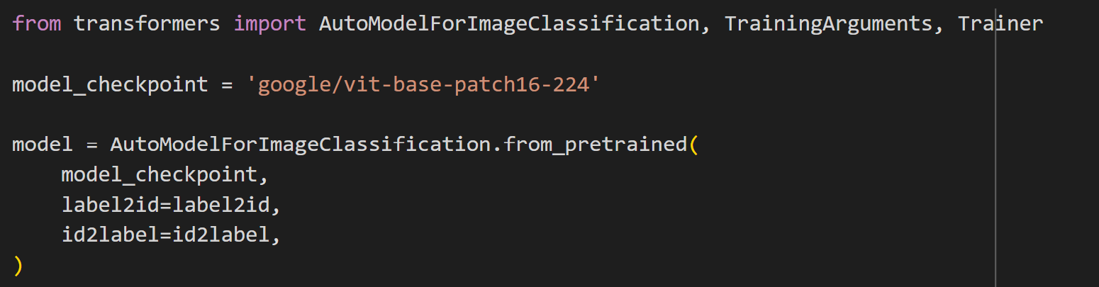
I used Hugging Face to instantiate a pre trained image classification model. For this case I used the Google ViT Patch 16 version. Hugging Face has a set of AutoModels that can be instantiated with a pre defined architecture and weights. Here we instantiate the Auto model for image classification because that is what we want to achieve.

Training was straight forward. I ran the training for 5 epochs (due to the small data size) using the default optimizer with a LR of 5e-5 and a CrossEntropy Loss.

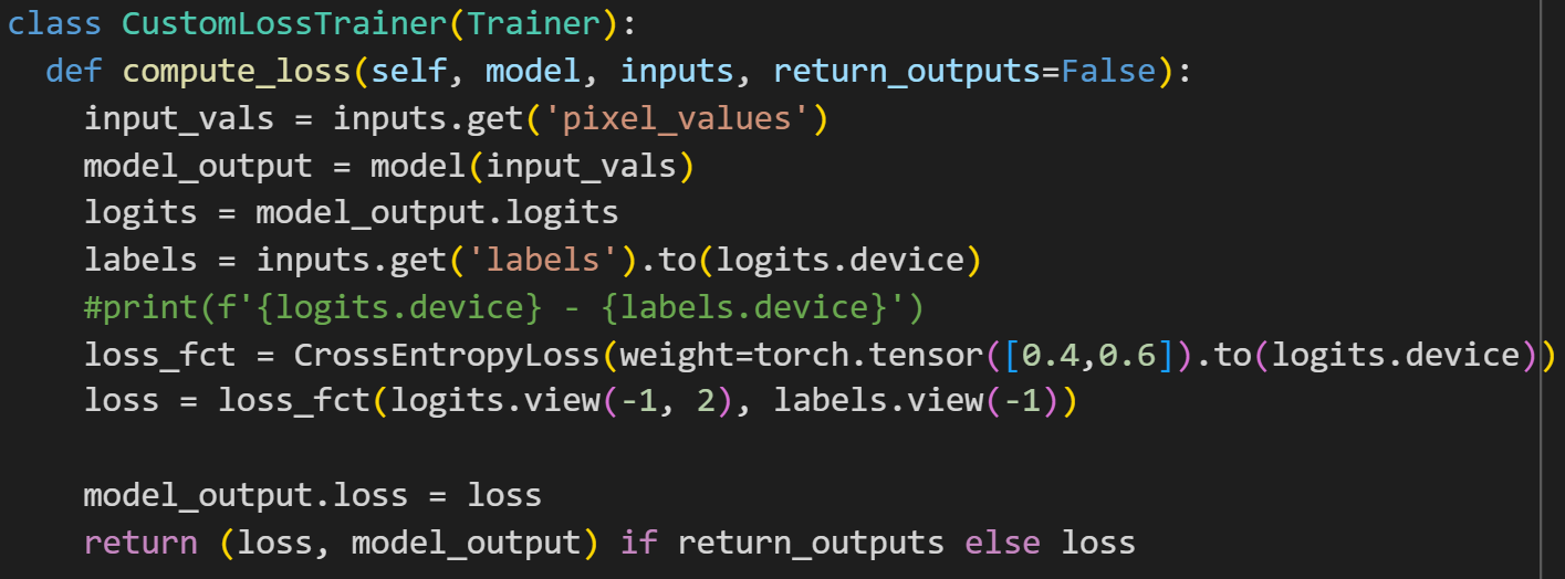
I also played around with a weighted loss function. Hugging Face’s trainers use inbuilt loss functions. To edit them you need to define your own custom loss function to override the one in the trainer. I used the standard Cross Entropy loss, but weighted it to pay more attention to the pictures of polyterasse as that is what I am interested in learning and to handle the class imbalance of my data set.

Inference

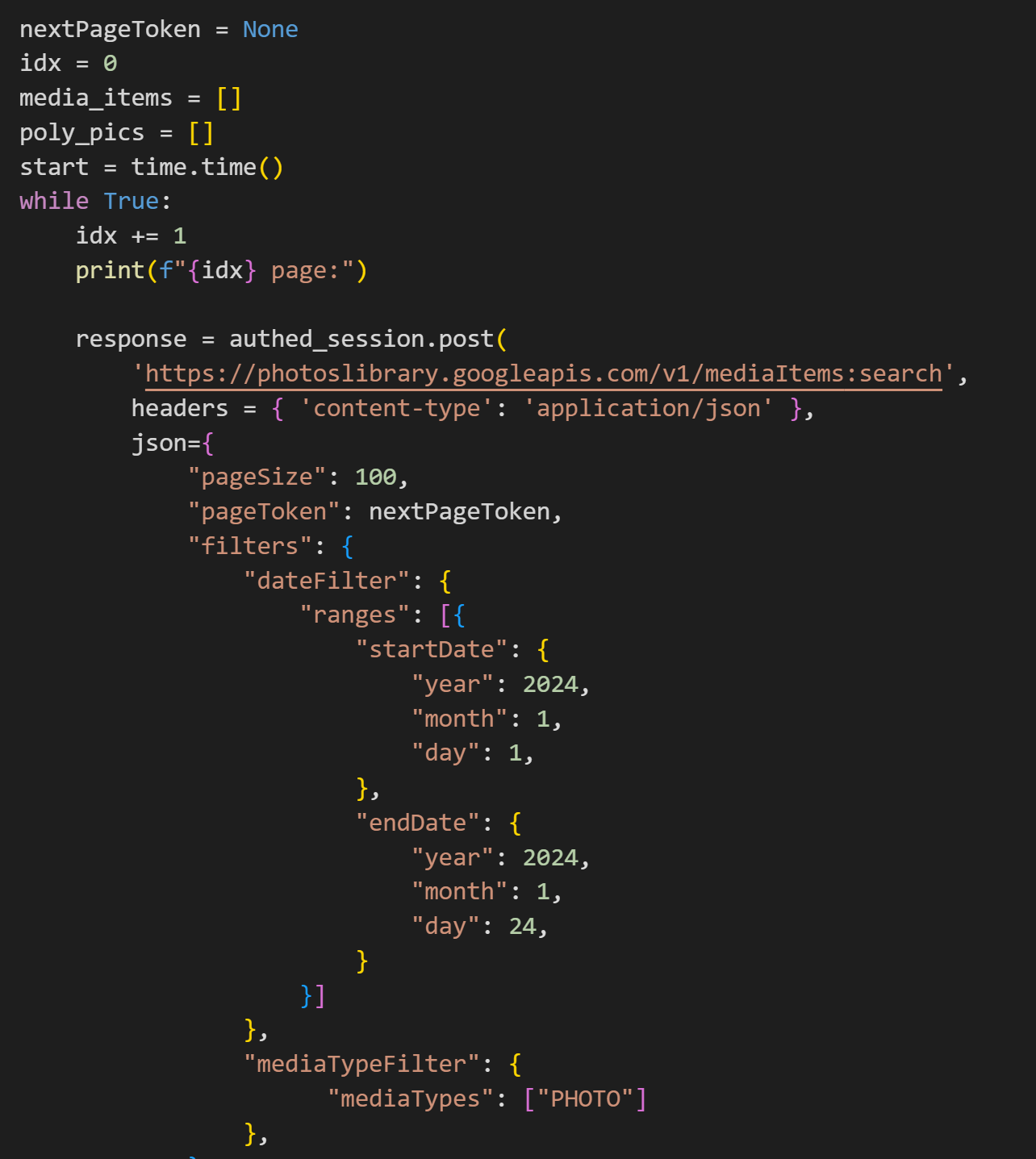
For the inference, I used the Google Photos API - MediaItems Search in order to fetch all photos from my library in a paginated manner, and then classify them using my model.

Results were unfortunately not great. A lot of unseen pictures were also being classified as pictures of Polyterasse - aka a lot of False Positives. In order to overcome this, I used a threshold in the final model output rather than using the argmax. This reduced the false positives to just a few.

I wanted to automatically add these classified pictures to an album in Google Photos, unfortunately the API only allows you to use the API to edit / move albums and pictures that were created via the API….. WHY GOOGLE WHY!! So I just manually added the photos to an album instead :P

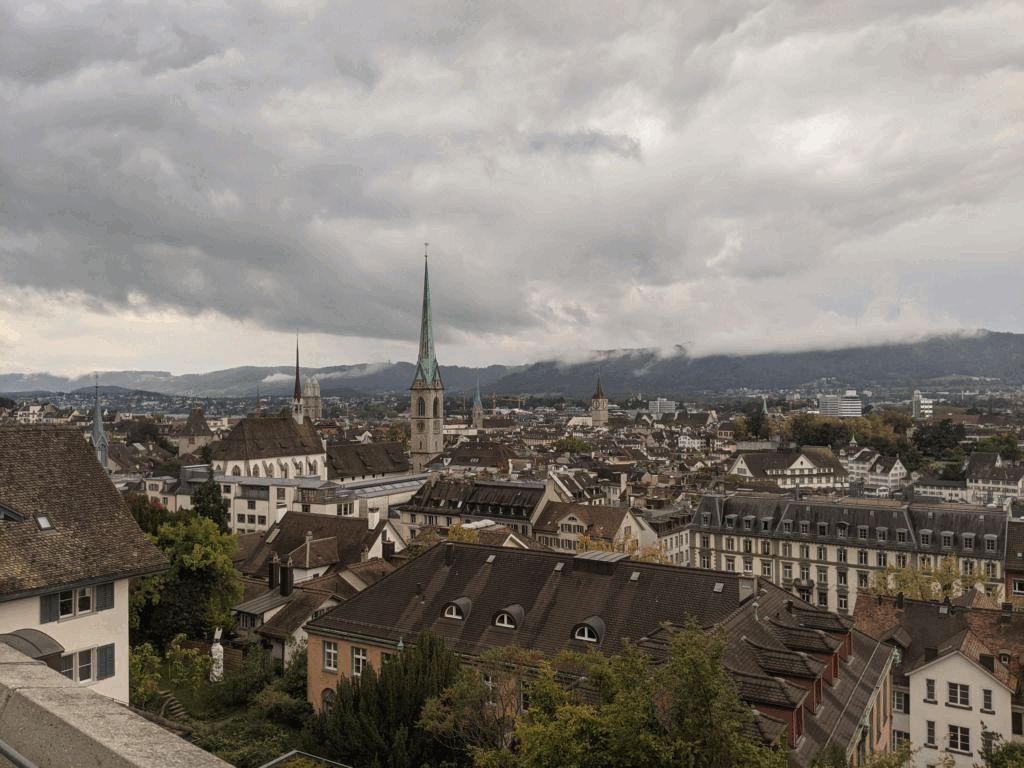
The final result was an album containing all my images of Polyterassee taken in the last two years, 8 of which are shown in the Image display above :D

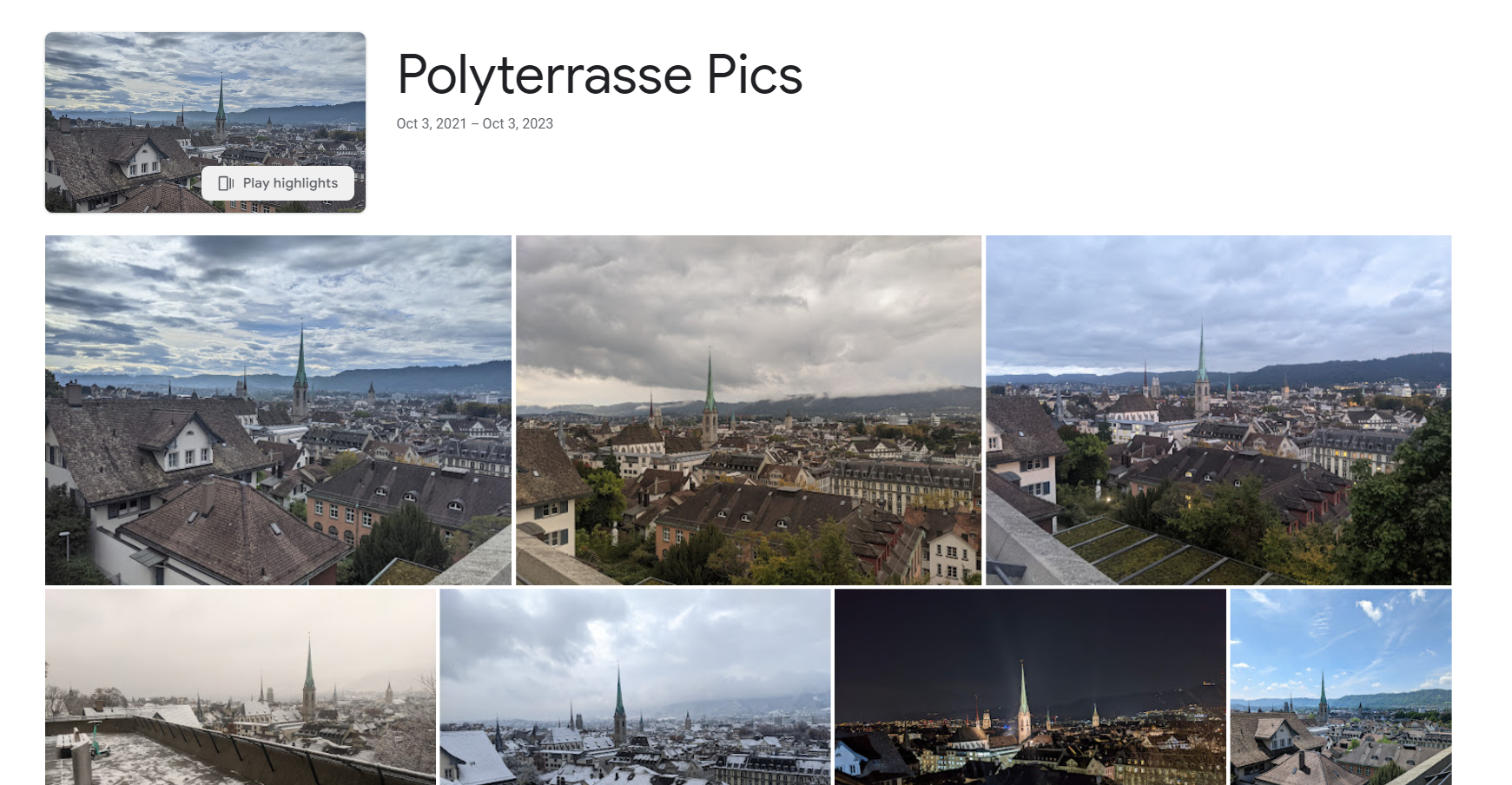
Photo Morphing

I wanted to play around with these images a bit more and tried to form a gif of them morphing from one to another. In order to do that I first trained an Auto Encoder to find the representation space, and then traverse this representation space in order to morph from one picture to another.

Auto Encoder

I used a convolutional auto encoder in order to find the representation space for these images as well as generate new intermediate representations. I took a subset of 16 different polyterasse images from my album and used them as the training set. Each image was used as the input and label, and MSE loss between the input and model output helped the model learn the correct representation. With around 200 epochs with an LR of 5e-4, the model was able to learn to regenerate the images quite well.

Now that I had learned the latent representation space, I could traverse the latent representation from one image to another and generate the intermediate images. So give the latent representations (l1 and l2) of two images (i1 and i2), I could move from l1 -> l2 by using a partial sum of the two like l3 = αl1 + (1-α)l2. Using this l3 value I could pass that into the auto encoder to decode that and generate an intermediate image.

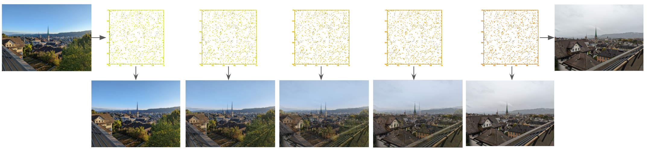
Using a set of 10 intermediate images, I took 5 different polyterasse pictures and then generated a gif looping through each of these images. The final output is as follows.

However this result was not as smooth as expected. The intermediate images looked very much like I just overlayed the two images and the parts never morphed cleanly. I would need to try something different.

Variational Auto Encoder

One point is that the generation of images is very mixed and not as continous. Variational Auto Encoders help solve that as they learn the latent space as a distribution instead of just a latent vector and hence can generate a more smoother image.

A few changes were to be made:

• I changed the latent space to just a 128 dimension vector. I reshaped the final output of the convolution encoder to a 128 length vector using a linear layer. In the decoder I used another linear layer to convert the latent representation back to the dimensions of the convolution output.
• The latent representation now has two vectors, one for the mean and the one for the log variance. model.encode(img) now returns mean and logvar of the latent representation of the image.
• The loss function now has another section. In addition to the reconstruction loss (MSE), we also want to minimize the distance (KL Divergence) between the learned distribution of the latent space with the actual representation. We do this by maximizing the ELBO or the estimated lower bound. The loss now becomes L = MSE - ELBO, which we then minimize.

Using a VAE we now get another model with smoother intermediate images.

Navigating the latent space

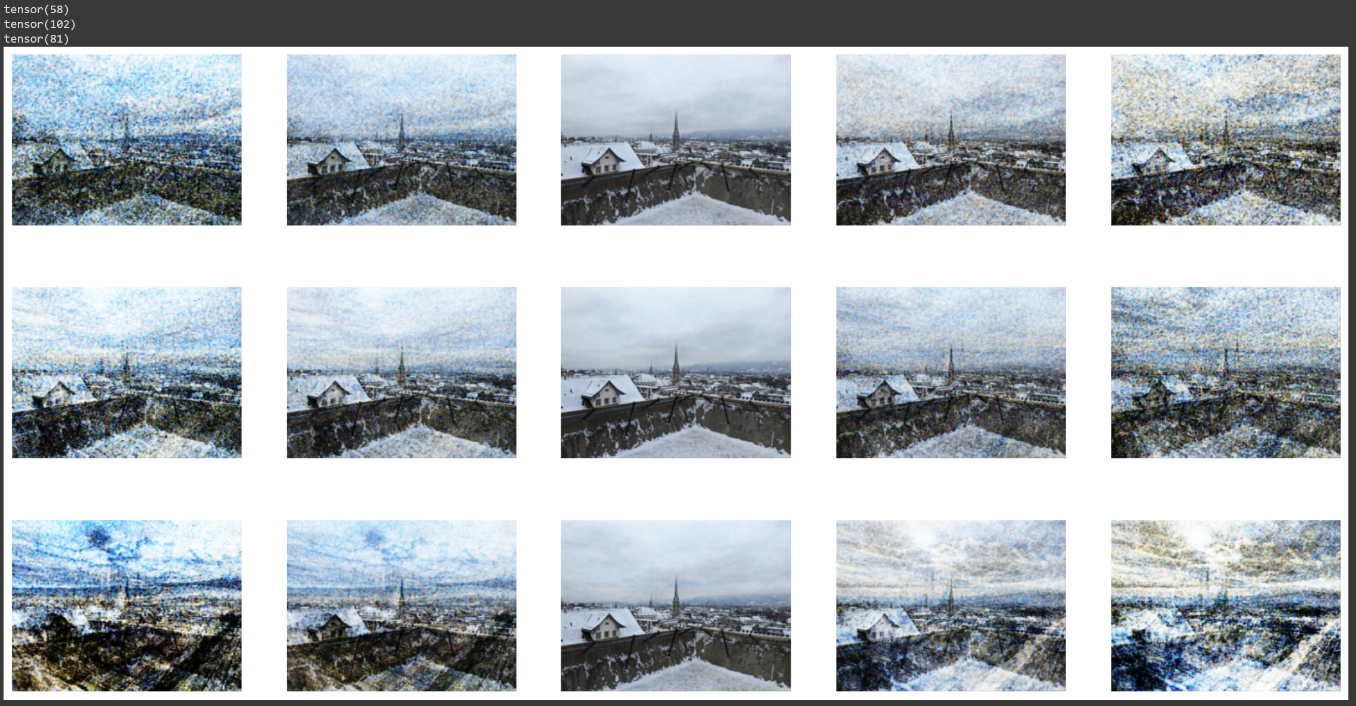
Moving directly from one representation to another seems to lead to messy intermediate images. To demonstrate this we try editing a single dimension in the latent space up and down.

When we take any dimension of the latent representation and move its value up or down, we see the generated images are messy.

Instead we want to find more meaningful directions to move the dimensions through. We do this by using PCA to find the most important vectors to move along. Principal Component Analysis or PCA, helps to identify the directions that explain the maximum variation between different values.

One drawback with out dataset is that we only have 16 images. Hence we have the latent space of 16 images, giving us a 16 x 128 matrix. Using PCA on this, we can get a max of 16 eigenvectors to explain the variation.

After performing PCA and getting the 16 eigenvectors, we can see the effect of the different principal components by looking at the eigenvalues for these different values. We can plot this in a ‘Scree plot’ that visually uses the contributions of the different eigen vectors to the value.

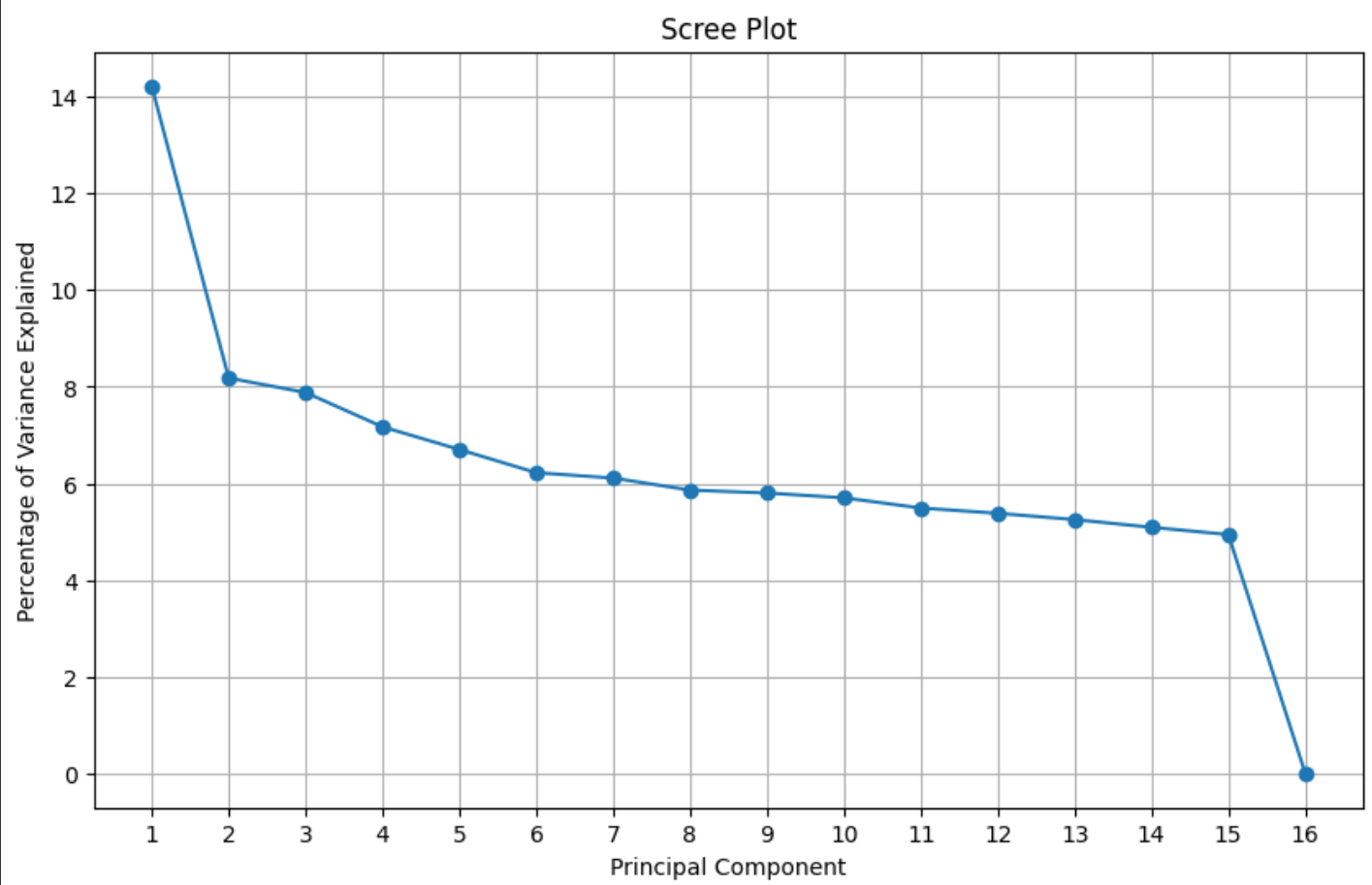
Ideally we want a few components to explain a lot of the variance. However in this case, we see the first component explains ~15% of the variance and the next 14 components explain the remainig 85% of the variance almost equally.

Still, we have a better direction to move along the latent space. If we look at the what happens when we move along the first three principal components, we see that each of the components seem to control a feature of the image better.

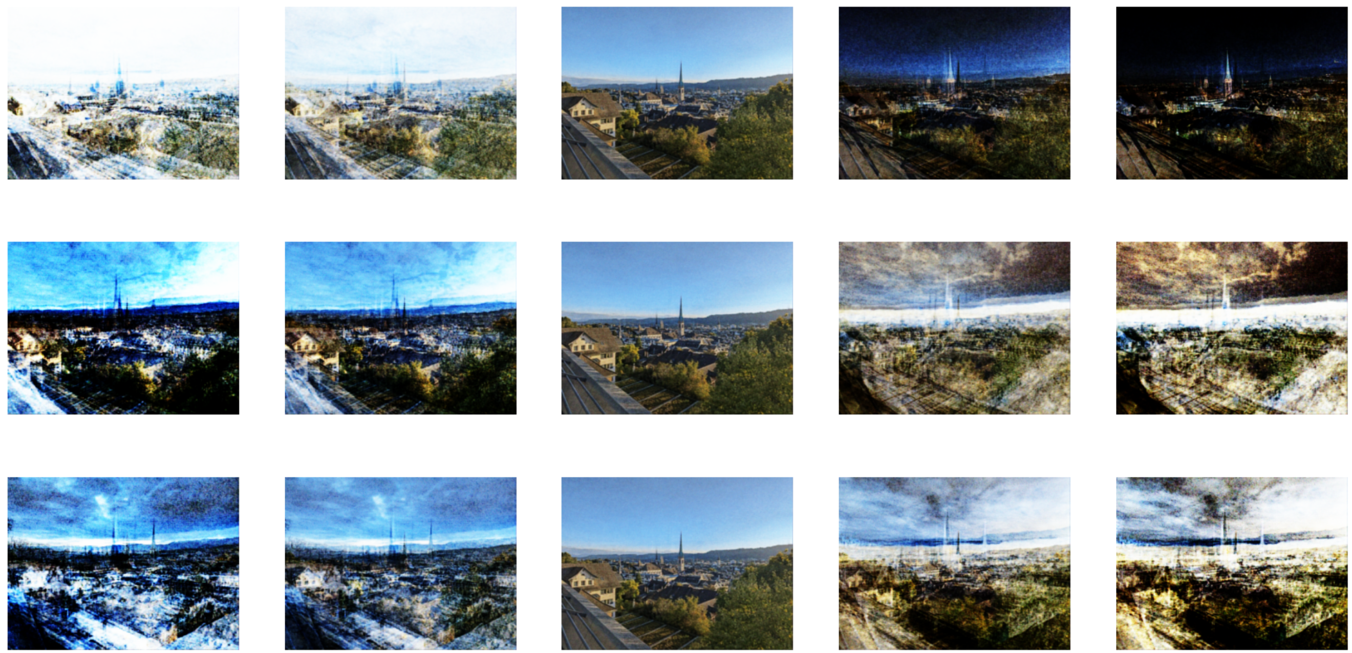
The first component looks to control the brightness in the image (between dark and bright, or more so night and day). The second and third seem to control the saturation as well as some structure shape at the bottom of the image. Trying to use these components to move along and generate the intermediate images we get a morph gif as below.

Unfortunately the morphing is still unclear and messy. I traversed the latent space once per eigen vector, hence there are now 15 intermediate images as compared to just 5 before and hence this might seem a bit smoother. However it does not capture the smooth morphing I would like to achieve. Still work to be done.

Back to the drawing board :)

To be continued….